Multi-Head Attention
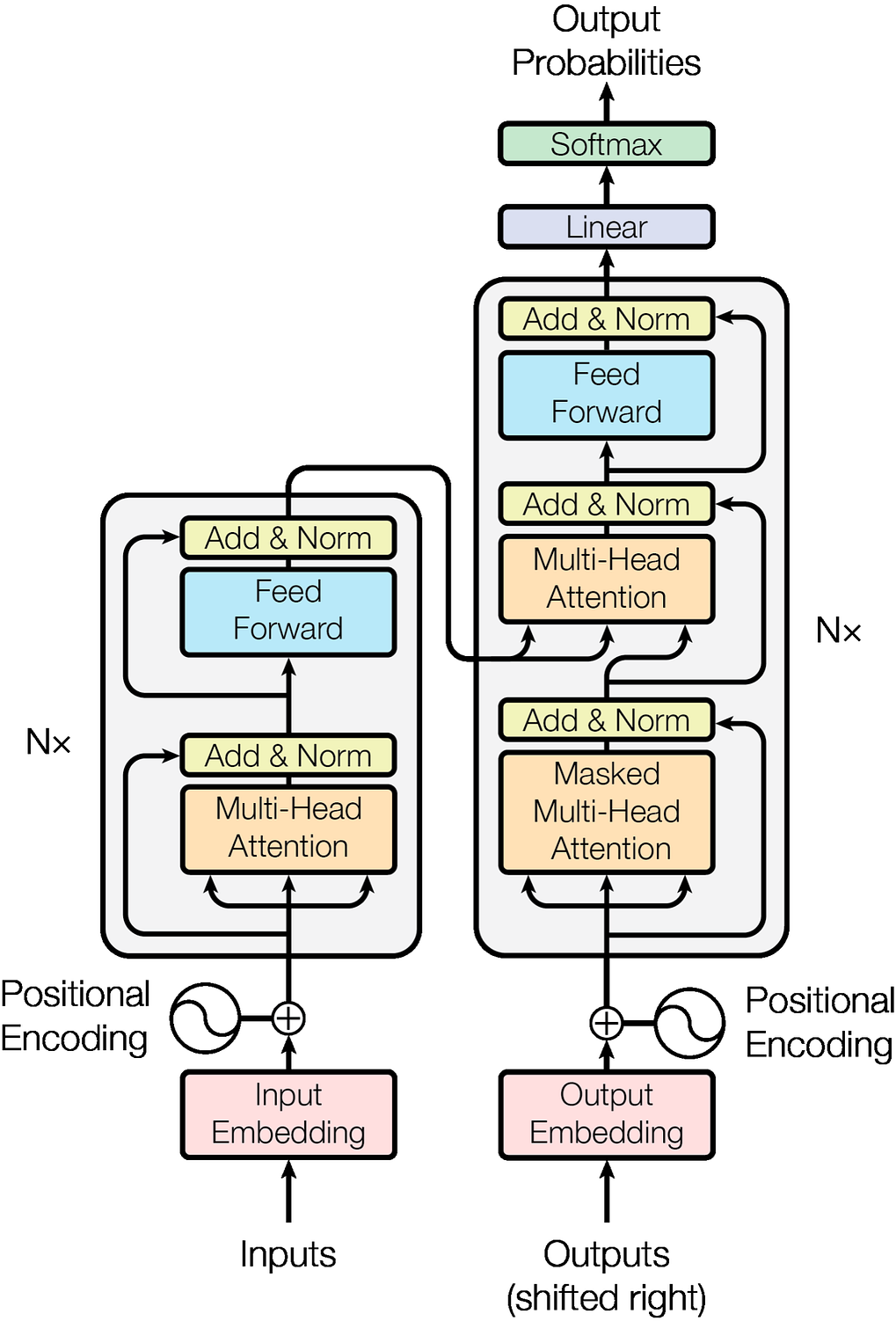
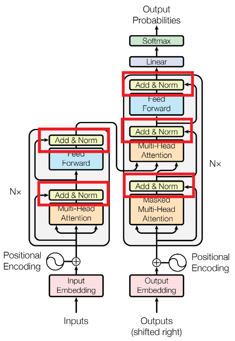
This article is the third in The Implemented Transformer series. It introduces the multi-head attention mechanism from scratch. Attention is the backbone and power behind transformers since it provides context for sequences.
Background
In transformers models, attention provides context for each sequence. This helps the model understand how different words relate to each other to create meaningful sentences. According to Wikipedia’s description, “the attention layer can access all previous states and weigh them according to a learned measure of relevance, providing relevant information about far-away tokens.”
To understand how it works, it would be best to have a sound understanding of the dot-product. For more information, see A Simple Introduction to the Dot Product. For more information on matrices and tensors, see A Simple Introduction to Tensors.
Multi-Head Attention
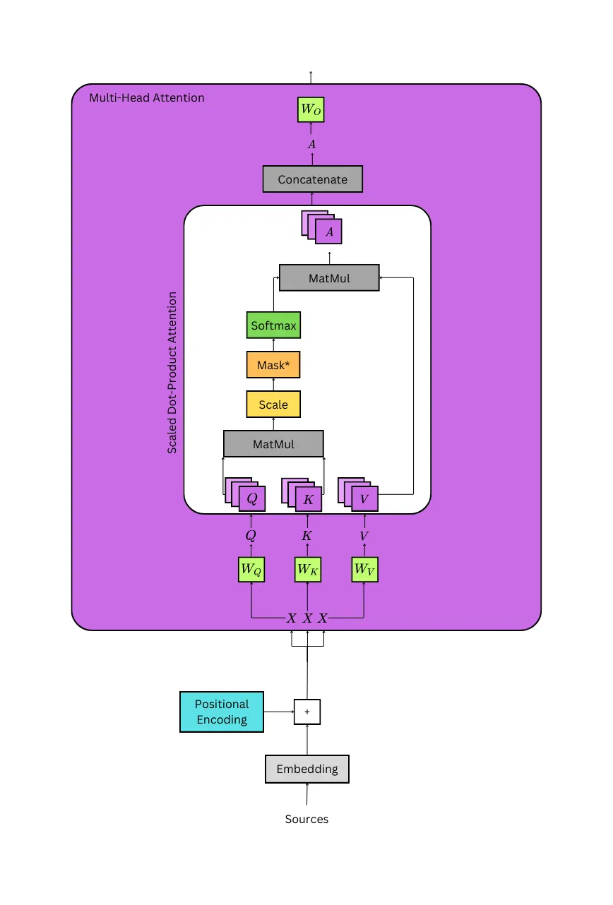
According to “Attention Is All You Need”:
An attention function can be described as mapping a query and a set of key-value pairs to an output, where the query, keys, values, and output are all vectors. The output is computed as a weighted sum of the values, where the weight assigned to each value is computed by a compatibility function of the query with the corresponding key.
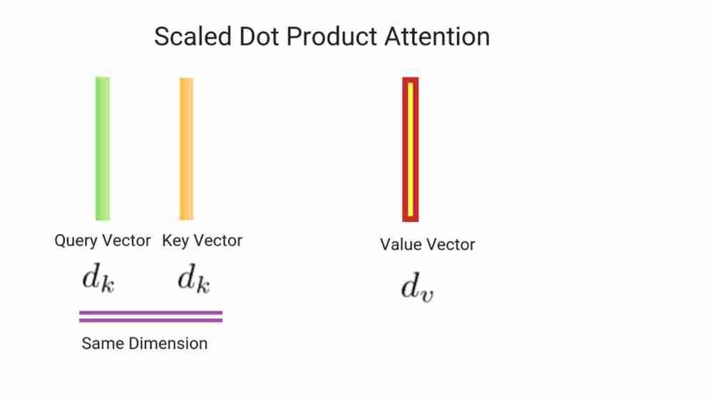
We call our particular attention “Scaled Dot-Product Attention”. The input consists of queries and keys of dimension d_key, and values of dimension d_value. We compute the dot products of the query with all keys, divide each by √(d_key), and apply a softmax function to obtain the weights on the values.
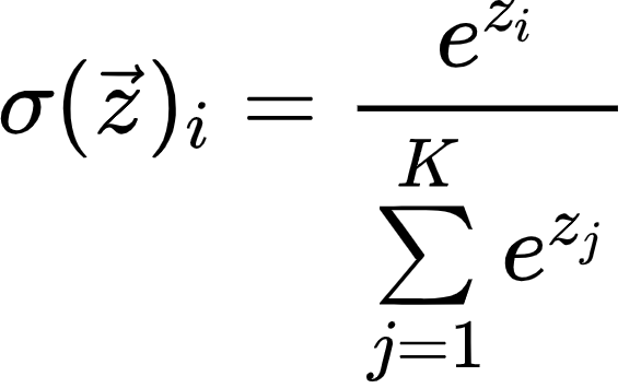
The model is scaled to avoid extremely small gradients resulting from the softmax function that can disrupt training. For more information about the softmax function, see A Simple Introduction to Softmax.
When multi-head attention is used, often d_key = d_value = (d_model / n_heads), where n_heads is the number of heads. Parallel attention layers are often used instead of the full-dimensionality because the model is able to “attend to information from different representation subspaces at different positions” according to the researchers. With only one head, averaging prevents this.
Passing the Input Through the Linear Layers
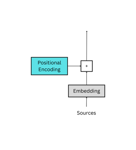
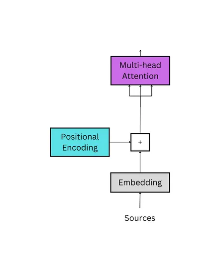
The first step to calculating attention is to acquire the Q, K, and V tensors; these are the query, key, and value tensors, respectively. They are calculated by taking the positionally encoded embeddings, which will be notated as X, and simultaneously passing the tensor through three linear layers, which are notated as Wq, Wk and Wv. This can be seen in the detailed image above.
- Q = XWq
- K = XWk
- V = XWv
To understand how the multiplication occurs, it is best to break down each component into its shape.
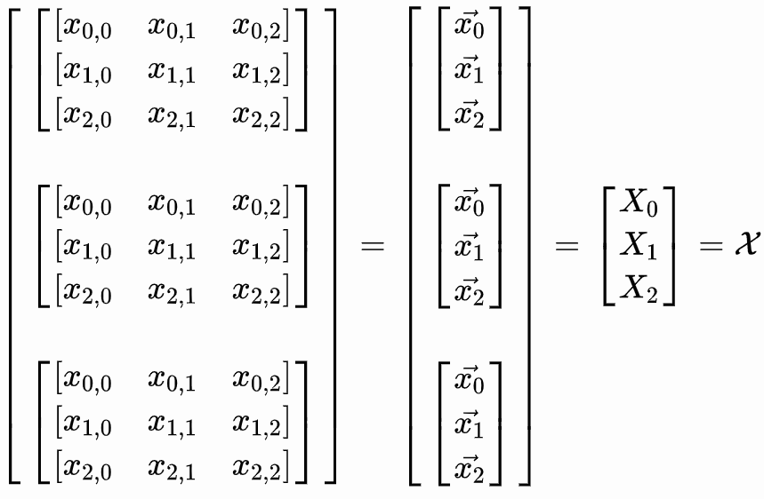
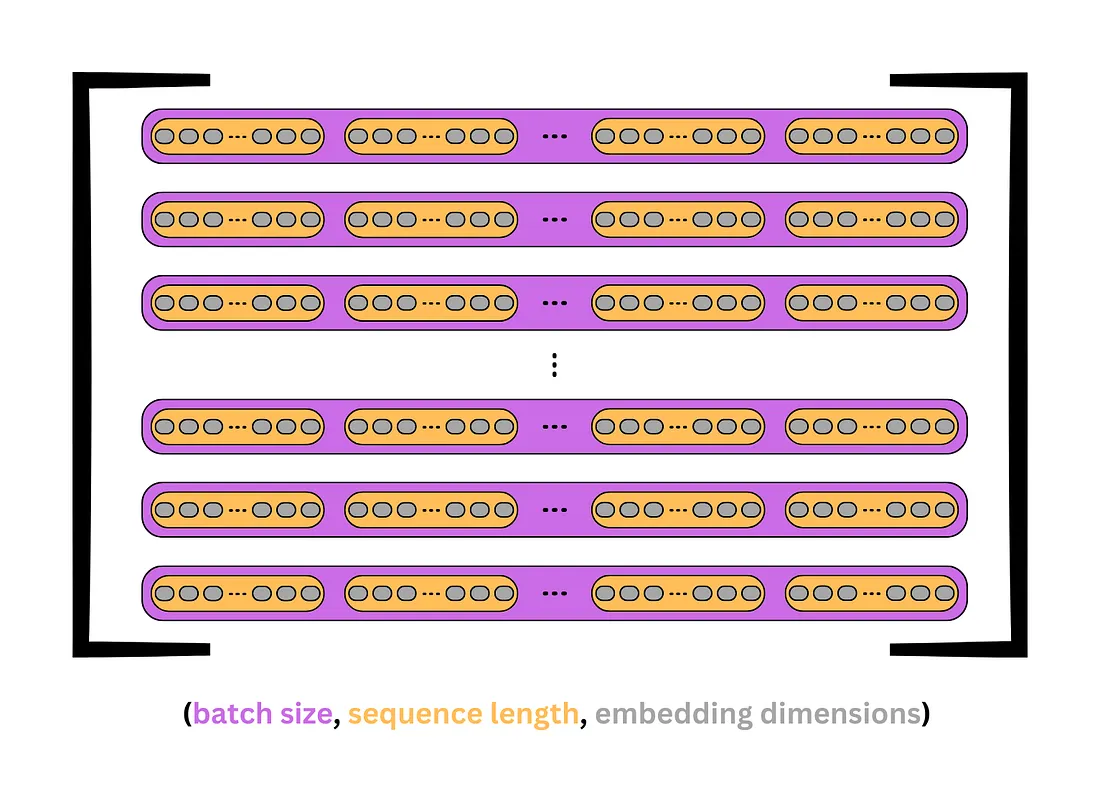
- X has a size of (batch_size, seq_length, d_model). An example would be a batch of 32 sequences of length 10 with an embedding of 512, which would have a shape of (32, 10, 512).
- Wq, Wk, and Wv have a size of (d_model, d_model). Following the example above, they would have a shape of (512, 512).
With this, the output of the multiplication can be better understood. Each weight matrix is broadcast across each sequence in the batch simultaneously to create the Q, K, and V tensors. For more information on broadcasting, see A Simple Introduction to Broadcasting.
- Q = XWq | (batch_size, seq_length, d_model) x (d_model, d_model) = (batch_size, seq_length, d_model)
- K = XWk | (batch_size, seq_length, d_model) x (d_model, d_model) = (batch_size, seq_length, d_model)
- V = XWv | (batch_size, seq_length, d_model) x (d_model, d_model) = (batch_size, seq_length, d_model)
The following image shows how Q, K, and V appear. Each purple box represents a sequence, and each orange box is a token or word in the sequence. The gray ovals represent the embeddings for each token.
The code below assumes the Positional Encoding and Embeddings classes are loaded from the previous articles of the series.
# convert the sequences to integers
sequences = ["I wonder what will come next!",
             "This is a basic example paragraph.",
             "Hello, what is a basic split?"]

# tokenize the sequences
tokenized_sequences = [tokenize(seq) for seq in sequences]

# index the sequences
indexed_sequences = [[stoi[word] for word in seq] for seq in tokenized_sequences]

# convert the sequences to a tensor
tensor_sequences = torch.tensor(indexed_sequences).long()

# vocab size
vocab_size = len(stoi)

# embedding dimensions
d_model = 8

# create the embeddings
lut = Embeddings(vocab_size, d_model) # look-up table (lut)

# create the positional encodings
pe = PositionalEncoding(d_model=d_model, dropout=0.1, max_length=10)

# embed the sequence
embeddings = lut(tensor_sequences)

# positionally encode the sequences
X = pe(embeddings)tensor([[[-3.45, -1.34, 4.12, -3.33, -0.81, -1.93, -0.28, 8.25],
[ 7.36, -1.09, 2.32, 1.52, 3.50, 1.42, 0.46, -0.95],
[-2.26, 0.53, -1.02, 1.49, -3.97, -2.19, 2.86, -0.59],
[-3.87, -2.02, 1.46, 6.78, 0.88, 1.08, -2.97, 1.45],
[ 1.12, -2.09, 1.19, 3.87, -0.00, 3.73, -0.88, 1.12],
[-0.35, -0.02, 3.98, -0.20, 7.05, 1.55, 0.00, -0.83]],
[[-4.27, 0.17, -2.08, 0.94, -6.35, 1.99, 5.23, 5.18],
[-0.00, -5.05, -7.19, 3.27, 1.49, -7.11, -0.59, 0.52],
[ 0.54, -2.33, -1.10, -2.02, -0.88, -3.15, 0.38, 5.26],
[ 0.87, -2.98, 2.67, 3.32, 1.16, 0.00, 1.74, 5.28],
[-5.58, -2.09, 0.96, -2.05, -4.23, 2.11, -0.00, 0.61],
[ 6.39, 2.15, -2.78, 2.45, 0.30, 1.58, 2.12, 3.20]],
[[ 4.51, -1.22, 2.04, 3.48, 1.63, 3.42, 1.21, 2.33],
[-2.34, 0.00, -1.13, 1.51, -3.99, -2.19, 2.86, -0.59],
[-4.65, -6.12, -7.08, 3.26, 1.50, -7.11, -0.59, 0.52],
[-0.32, -2.97, -0.99, -2.05, -0.87, -0.00, 0.39, 5.26],
[-0.12, -2.61, 2.77, 3.28, 1.17, 0.00, 1.74, 5.28],
[-5.64, 0.49, 2.32, -0.00, -0.44, 4.06, 3.33, 3.11]]],
grad_fn=<MulBackward0>)At this point, the embedded sequences, X, have a shape of (3, 6, 8). There are 3 sequences of 6 tokens with an 8 dimensional embedding.
The linear layers for Wq, Wk, and Wv can be created using nn.Linear(d_model, d_model). This creates an (8,8) matrix that will be broadcast during multiplication across each sequence.
Wq = nn.Linear(d_model, d_model)          # query weights (8,8)
Wk = nn.Linear(d_model, d_model)          # key weights   (8,8)
Wv = nn.Linear(d_model, d_model)          # value weights (8,8)

Wq.state_dict()['weight']
tensor([[ 0.19, 0.34, -0.12, -0.22, 0.26, -0.06, 0.12, -0.28],
[ 0.09, 0.22, 0.32, 0.11, 0.21, 0.03, -0.35, 0.31],
[-0.34, -0.21, -0.11, 0.34, -0.28, 0.03, 0.26, -0.22],
[-0.35, 0.11, 0.17, 0.21, -0.19, -0.29, 0.22, 0.20],
[ 0.19, 0.04, -0.07, -0.02, 0.01, -0.20, 0.30, -0.19],
[ 0.23, 0.15, 0.22, 0.26, 0.17, 0.16, 0.23, 0.18],
[ 0.01, 0.06, -0.31, 0.19, 0.22, 0.08, 0.15, -0.04],
[-0.11, 0.24, -0.20, 0.26, -0.01, -0.14, 0.29, -0.32]])The weights for Wq can be seen above. Wk and Wv have the same shapes with different weights. When X is passed through each linear layer, it retains its shape, but now Q, K, and V have been transformed by the weights into unique tensors.
Q = Wq(X) # (3,6,8)x(broadcast 8,8) = (3,6,8)
K = Wk(X) # (3,6,8)x(broadcast 8,8) = (3,6,8)
V = Wv(X) # (3,6,8)x(broadcast 8,8) = (3,6,8)

Q
tensor([
# sequence 0
[[-3.13, 2.71, -2.07, 3.54, -2.25, -0.26, -2.80, -4.31],
[ 1.70, 1.63, -2.90, -2.90, 1.15, 3.01, 0.49, -1.14],
[-0.69, -2.38, 3.00, 3.09, 0.97, -0.98, -0.10, 2.16],
[-3.52, 2.08, 2.36, 2.16, -2.48, 0.58, 0.33, -0.26],
[-1.99, 1.18, 0.64, -0.45, -1.32, 1.61, 0.28, -1.18],
[ 1.66, 2.46, -2.39, -0.97, -0.47, 1.83, 0.36, -1.06]],
# sequence 1
[[-3.13, -2.43, 3.85, 4.34, -0.60, -0.03, 0.04, 0.62],
[-0.82, -2.67, 1.82, 0.89, 1.30, -2.65, 2.01, 1.56],
[-1.42, 0.11, -1.40, 1.36, -0.21, -0.87, -0.88, -2.24],
[-2.70, 1.88, -0.10, 1.95, -0.75, 2.54, -0.14, -1.91],
[-2.67, -1.58, 2.46, 1.93, -1.78, -2.44, -1.76, -1.23],
[ 1.23, 0.78, -1.93, -1.12, 1.07, 2.98, 1.82, 0.18]],
# sequence 2
[[-0.71, 1.90, -1.12, -0.97, -0.23, 3.54, 0.65, -1.39],
[-0.87, -2.54, 3.16, 3.04, 0.94, -1.10, -0.10, 2.07],
[-2.06, -3.30, 3.63, 2.39, 0.38, -3.87, 1.86, 1.79],
[-2.00, 0.02, -0.90, 0.68, -1.03, -0.63, -0.70, -2.77],
[-2.76, 1.90, 0.14, 2.34, -0.93, 2.38, -0.17, -1.75],
[-1.82, 0.15, 1.79, 2.87, -1.65, 0.97, -0.21, -0.54]]],
grad_fn=<ViewBackward0>)Q, K, and V all have this shape. Like before, each matrix is a sequence, and each row is a token represented by embeddings.
Splitting Q, K, and V Into Their Heads
With the Q, K, and V tensors created, they can now be split into their respective heads by changing the view of d_model to (n_heads, d_key). n_heads can be an arbitrary number, but it is common to do 8, 10, or 12 when working with larger embeddings. Remember that d_key = (d_model / n_heads).
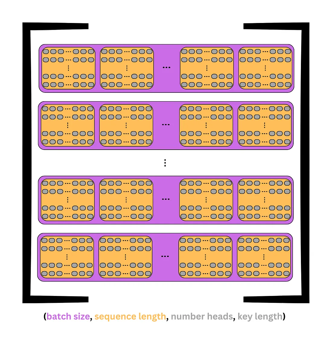
In the previous image, each token contained d_model embeddings in a single dimension. Now, this dimension is split into rows and columns to create a matrix; each row is a head containing keys. This can be seen in the image above.
The shape of each tensor becomes:
- (batch_size, seq_length, d_model) → (batch_size, seq_length, n_heads, d_key)
Assuming four heads were chosen for the example, the (3, 6, 8) tensors would be split into (3, 6, 4, 2) tensors, where there are 3 sequences, 6 tokens in each sequence, 4 heads in each token, and 2 elements in each head.
This can be done with view, which can be used to add and set the size of each dimension. Since the batch size, or number of sequences, is the same for each example, the batch size can be set. Likewise, the number of heads and number of keys should be constant across each tensor. -1 can be used to represent the leftover values, which are the sequence length.
batch_size = Q.size(0)
n_heads = 4
d_key = d_model//n_heads # 8/4 = 2

# query tensor | -1 = query_length | (3, 6, 8) -> (3, 6, 4, 2)
Q = Q.view(batch_size, -1, n_heads, d_key)

# value tensor | -1 = key_length | (3, 6, 8) -> (3, 6, 4, 2)
K = K.view(batch_size, -1, n_heads, d_key)

# value tensor | -1 = value_length | (3, 6, 8) -> (3, 6, 4, 2)
V = V.view(batch_size, -1, n_heads, d_key)

Q
Below is the Q tensor as an example. Each of the 3 sequences has 6 tokens, and each token is a matrix with 4 heads (rows) and 2 keys in each head.
tensor([
        # sequence 0
        [[[-3.13,  2.71],
          [-2.07,  3.54],
          [-2.25, -0.26],
          [-2.80, -4.31]],

         [[ 1.70,  1.63],
          [-2.90, -2.90],
          [ 1.15,  3.01],
          [ 0.49, -1.14]],

         [[-0.69, -2.38],
          [ 3.00,  3.09],
          [ 0.97, -0.98],
          [-0.10,  2.16]],

         [[-3.52,  2.08],
          [ 2.36,  2.16],
          [-2.48,  0.58],
          [ 0.33, -0.26]],

         [[-1.99,  1.18],
          [ 0.64, -0.45],
          [-1.32,  1.61],
          [ 0.28, -1.18]],

         [[ 1.66,  2.46],
          [-2.39, -0.97],
          [-0.47,  1.83],
          [ 0.36, -1.06]]],

        # sequence 1
        [[[-3.13, -2.43],
          [ 3.85,  4.34],
          [-0.60, -0.03],
          [ 0.04,  0.62]],

         [[-0.82, -2.67],
          [ 1.82,  0.89],
          [ 1.30, -2.65],
          [ 2.01,  1.56]],

         [[-1.42,  0.11],
          [-1.40,  1.36],
          [-0.21, -0.87],
          [-0.88, -2.24]],

         [[-2.70,  1.88],
          [-0.10,  1.95],
          [-0.75,  2.54],
          [-0.14, -1.91]],

         [[-2.67, -1.58],
          [ 2.46,  1.93],
          [-1.78, -2.44],
          [-1.76, -1.23]],

         [[ 1.23,  0.78],
          [-1.93, -1.12],
          [ 1.07,  2.98],
          [ 1.82,  0.18]]],

        # sequence 2
        [[[-0.71,  1.90],
          [-1.12, -0.97],
          [-0.23,  3.54],
          [ 0.65, -1.39]],

         [[-0.87, -2.54],
          [ 3.16,  3.04],
          [ 0.94, -1.10],
          [-0.10,  2.07]],

         [[-2.06, -3.30],
          [ 3.63,  2.39],
          [ 0.38, -3.87],
          [ 1.86,  1.79]],

         [[-2.00,  0.02],
          [-0.90,  0.68],
          [-1.03, -0.63],
          [-0.70, -2.77]],

         [[-2.76,  1.90],
          [ 0.14,  2.34],
          [-0.93,  2.38],
          [-0.17, -1.75]],

         [[-1.82,  0.15],
          [ 1.79,  2.87],
          [-1.65,  0.97],
          [-0.21, -0.54]]]], grad_fn=<ViewBackward0>)
To proceed, it would be best to transpose seq_length and n_heads, the second and third dimensions, to have the following shape:
- (batch_size, seq_length, n_heads, d_key) → (batch_size, n_heads, seq_length, d_key)
Now, each sequence is split across n_heads, with each head receiving seq_length tokens with d_key elements in each token instead of d_model. This achieves the researchers’ goal to “attend to information from different representation subspaces at different positions.”
A visualization of this tensor can be seen in the image below. Each sequence is purple, and each head is gray. Within the heads, each token is a row of d_key elements.
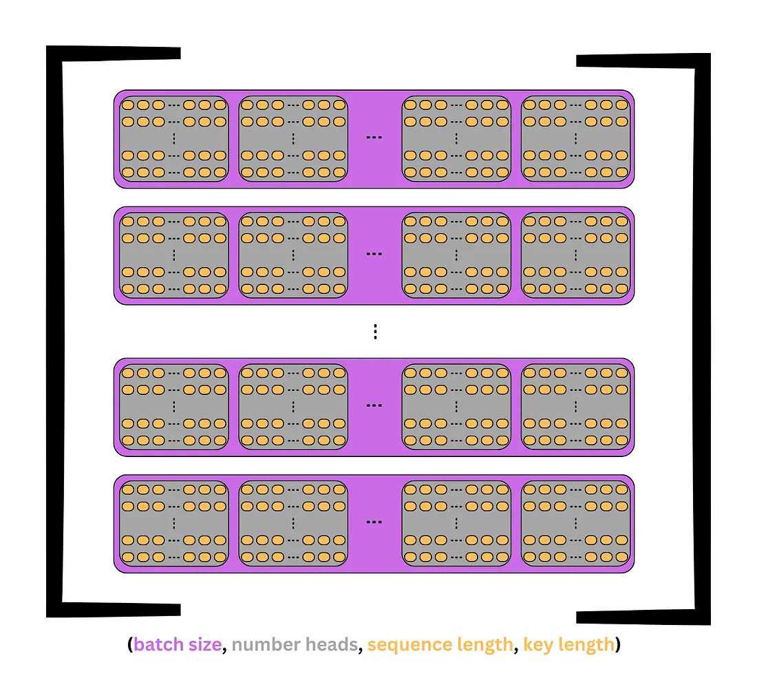
To return to the previous example, the Q tensor would be transposed from (3, 6, 4, 2) to (3, 4, 6, 2). This tensor would now represent 3 sequences, with each split across n_heads = 4, with each head containing seq_length = 6 tokens, each with a d_key = 2 element key.
Essentially, each head contains a copy of each sequence’s tokens, but it only has a d_key = 2 element representation instead of the full d_model = 8 element representation. This means each sequence is represented in n_head = 4 different subspaces simultaneously.
The code below uses permute to switch the second and third axes for each tensor.
# query tensor | (3, 6, 4, 2) -> (3, 4, 6, 2)
Q = Q.permute(0, 2, 1, 3)
# key tensor | (3, 6, 4, 2) -> (3, 4, 6, 2)
K = K.permute(0, 2, 1, 3)
# value tensor | (3, 6, 4, 2) -> (3, 4, 6, 2)
V = V.permute(0, 2, 1, 3)

Q
tensor([
# sequence 0
[[[-3.13, 2.71],
[ 1.70, 1.63],
[-0.69, -2.38],
[-3.52, 2.08],
[-1.99, 1.18],
[ 1.66, 2.46]],
[[-2.07, 3.54],
[-2.90, -2.90],
[ 3.00, 3.09],
[ 2.36, 2.16],
[ 0.64, -0.45],
[-2.39, -0.97]],
[[-2.25, -0.26],
[ 1.15, 3.01],
[ 0.97, -0.98],
[-2.48, 0.58],
[-1.32, 1.61],
[-0.47, 1.83]],
[[-2.80, -4.31],
[ 0.49, -1.14],
[-0.10, 2.16],
[ 0.33, -0.26],
[ 0.28, -1.18],
[ 0.36, -1.06]]],
# sequence 1
[[[-3.13, -2.43],
[-0.82, -2.67],
[-1.42, 0.11],
[-2.70, 1.88],
[-2.67, -1.58],
[ 1.23, 0.78]],
[[ 3.85, 4.34],
[ 1.82, 0.89],
[-1.40, 1.36],
[-0.10, 1.95],
[ 2.46, 1.93],
[-1.93, -1.12]],
[[-0.60, -0.03],
[ 1.30, -2.65],
[-0.21, -0.87],
[-0.75, 2.54],
[-1.78, -2.44],
[ 1.07, 2.98]],
[[ 0.04, 0.62],
[ 2.01, 1.56],
[-0.88, -2.24],
[-0.14, -1.91],
[-1.76, -1.23],
[ 1.82, 0.18]]],
# sequence 2
[[[-0.71, 1.90],
[-0.87, -2.54],
[-2.06, -3.30],
[-2.00, 0.02],
[-2.76, 1.90],
[-1.82, 0.15]],
[[-1.12, -0.97],
[ 3.16, 3.04],
[ 3.63, 2.39],
[-0.90, 0.68],
[ 0.14, 2.34],
[ 1.79, 2.87]],
[[-0.23, 3.54],
[ 0.94, -1.10],
[ 0.38, -3.87],
[-1.03, -0.63],
[-0.93, 2.38],
[-1.65, 0.97]],
[[ 0.65, -1.39],
[-0.10, 2.07],
[ 1.86, 1.79],
[-0.70, -2.77],
[-0.17, -1.75],
[-0.21, -0.54]]]], grad_fn=<PermuteBackward0>)While it is nice to have the full view, it would easier to understand by examining a single sequence.
It is easy to see the four heads in this single sequence. Each head contains six rows, which are the tokens, and each row has two elements, which are the keys. This shows how the sequence is split across four subspaces to create different representations of the same sequence.
# select the first sequence from the Query tensor
Q[0]
tensor([
# head 0
[[-3.13, 2.71],
[ 1.70, 1.63],
[-0.69, -2.38],
[-3.52, 2.08],
[-1.99, 1.18],
[ 1.66, 2.46]],
# head 1
[[-2.07, 3.54],
[-2.90, -2.90],
[ 3.00, 3.09],
[ 2.36, 2.16],
[ 0.64, -0.45],
[-2.39, -0.97]],
# head 2
[[-2.25, -0.26],
[ 1.15, 3.01],
[ 0.97, -0.98],
[-2.48, 0.58],
[-1.32, 1.61],
[-0.47, 1.83]],
# head 3
[[-2.80, -4.31],
[ 0.49, -1.14],
[-0.10, 2.16],
[ 0.33, -0.26],
[ 0.28, -1.18],
[ 0.36, -1.06]]], grad_fn=<SelectBackward0>)Calculating Attention

With Q, K, and V split into their heads, the scaled-dot product of Q and K can now be computed. The equation above shows that the first step is to perform tensor multiplication. However, K has to be transposed first.
Moving forward, the seq_length shape of each tensor will be known by its respective tensor for clarity, Q_length, K_length, or V_length:
- Q has a shape of (batch_size, n_heads, Q_length, d_key)
- K has a shape of (batch_size, n_heads, K_length, d_key)
- V has a shape of (batch_size, n_heads, V_length, d_key)
The two rightmost dimensions of K must be transposed to change the shape to (batch_size, n_heads, d_key, K_length).
Now, the output of QK^T will be:
- (batch_size, n_heads, Q_length, d_key) x (batch_size, n_heads, d_key, K_length) = (batch_size, n_heads, Q_length, K_length)
The corresponding sequences in each tensor will be multiplied against each other. The first sequence in Q will be multiplied with the first sequence in K, the second sequence in Q with the second sequence in K, and so on. When these sequences are multiplied against each other, each head will be multiplied against its corresponding head in the opposite tensor. The first head of the first sequence of Q will be multiplied against the first head of the first sequence of K, the second head of the first sequence of Q with the second head of the first sequence of K, and so on. While multiplying these heads, each token in Q’s head, with a shape of (Q_length, d_key), is multiplied against each token in K’s head, with a shape of (d_key, K_length). The result is a (Q_length, K_length) matrix that shows the strength of each word with every other word including itself. This is where the name “self-attention” comes from since the model finds which words are the most relevant to the sequence by multiplying it with another representation of itself.
QK^T is scaled by d_key to help make the output of the softmax function in the next step less focused around 0 and 1. Values closer to zero and one in the unscaled distribution get closer to the middle of the distribution. This can be seen in the demonstration in the appendix.
Continuing the example, the output of the scaled dot product has a shape of (3, 4, 6, 2) x (3, 4, 2, 6) = (3, 4, 6, 6).
# calculate scaled dot product
scaled_dot_prod = torch.matmul(Q, K.permute(0, 1, 3, 2)) / math.sqrt(d_key) # (batch_size, n_heads, Q_length, K_length)
This tensor is then passed through the softmax function to create a probability distribution. Please note how softmax is applied over each row of each matrix in each head. The softmax dimension can be set to either -1 or 3 since both indicate the rightmost dimension in the shape, which are the keys. As a reminder, for more information about softmax, see A Simple Introduction to Softmax.
# apply softmax to get context for each token and others
attn_probs = torch.softmax(scaled_dot_prod, dim=-1) # (batch_size, n_heads, Q_length, K_length)
These attention probabilities can be visualized using imshow from matplotlib. A function to display all the heads of a sequence simultaneously can be found in the appendix, called display_attention. White is closer to 1, and black is closer to 0.
# sequence 0
display_attention(["i", "wonder", "what", "will", "come", "next"],
                  ["i", "wonder", "what", "will", "come", "next"],
                  attn_probs[0], 4, 2, 2)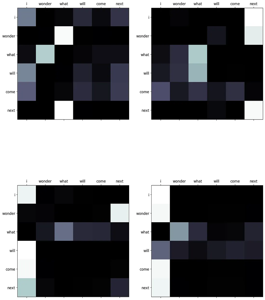
# sequence 1
display_attention(["this", "is", "a", "basic", "example", "paragraph"],
                  ["this", "is", "a", "basic", "example", "paragraph"],
                  attn_probs[1], 4, 2, 2)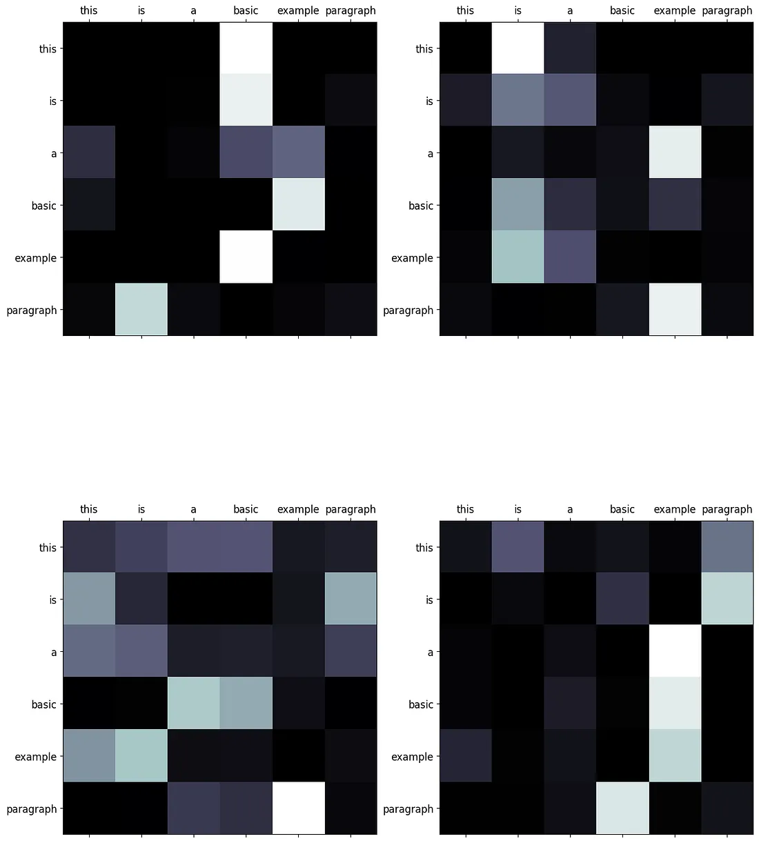
# sequence 2
display_attention(["hello", "what", "is", "a", "basic", "split"],
                  ["hello", "what", "is", "a", "basic", "split"],
                  attn_probs[2], 4, 2, 2)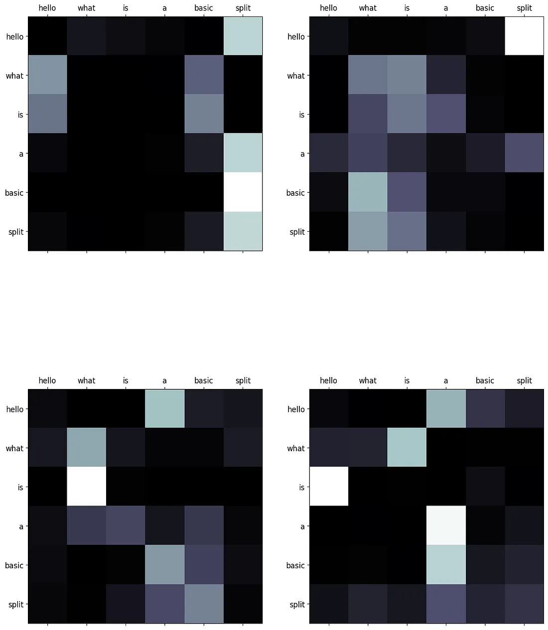
These demonstrate the relationship between each query (row) and key (column). Each intersection between words in the sequence represent the strength of the relationship. Since these values are generated from random weights, they do not show any valid relationships as of now. The image below demonstrates how these matrices would look if the encoder was trained.

With these probabilities calculated, the next step is to multiply them with the V tensor to create a summary of these distributions. The context for each word is essentially aggregated.
When this occurs, the shape of the tensor returns to normal.

# multiply attention and values to get reweighted values
A = torch.matmul(attn_probs, V) # (batch_size, n_heads, Q_length, d_key)
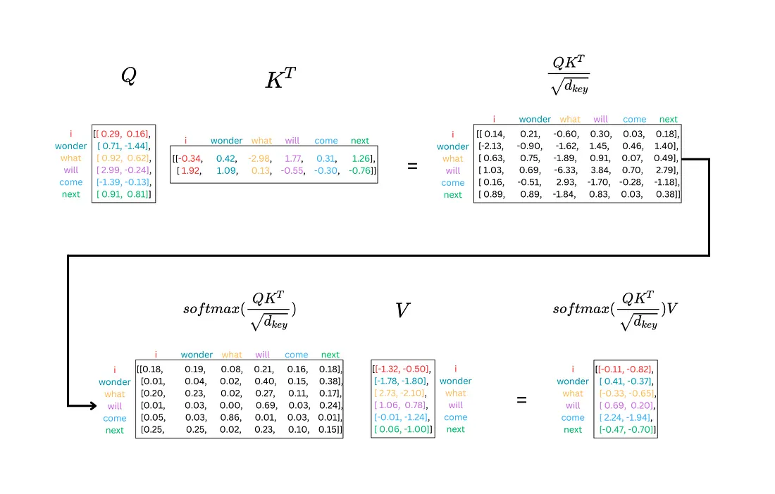
Below is a diagram that follows each of these steps for this example.
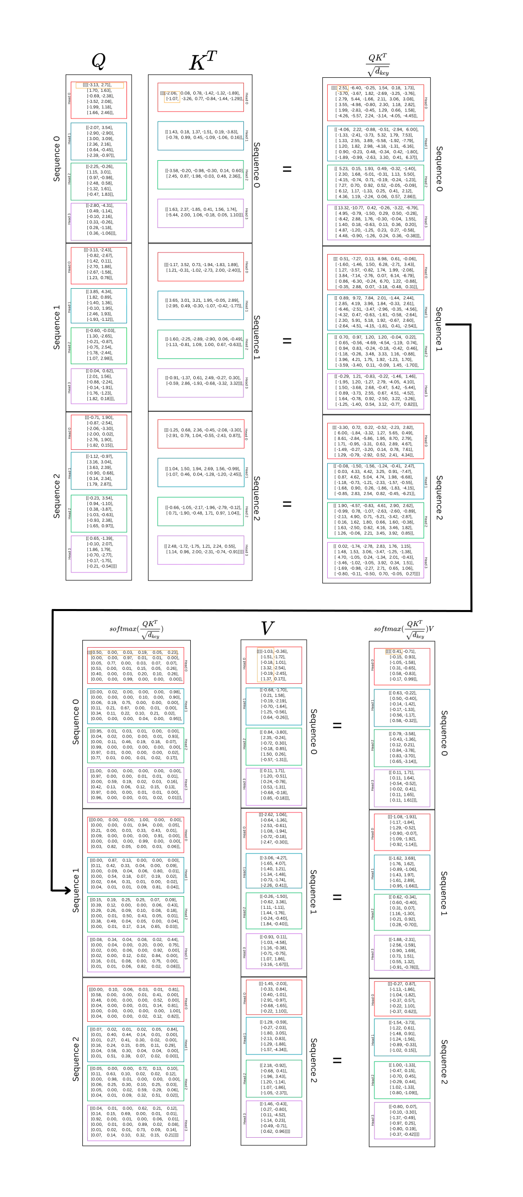
What exactly is happening here? Well, Q and K are both representations of the same sequences broken into query and key components across different heads. This calculates the relation between each word in the sequence with every other word in the sequence. This occurs across n_heads subspaces. The dot product between the query representation of each word and the key representation of each word is calculated. This indicates the “strength” or “weight” between each word and the other words. With training, this strength will help the model understand which words should have a higher “weight” between them; this will indicate which words are most important for context and prediction. To emphasize again, the query is multiplied with the key to generate a weight between each token and all the other tokens in the sequence.
Each row in the softmax tensor represents a token’s relationship to every other token within the same sequence. In V, each column is a representation of the sequence. The two tensors are multiplied together to reweight the values and calculate a summary of the most important context for each token in each head or subspace.
The diagram below follows the self-attention of a single head in a sequence.
Passing It Through the Output Layer
At this point, the heads can be concatenated back together before they are passed through the final linear layer, Wo in the multi-head attention mechanism.
The concatenation reverses the split that was performed originally. The first step is to transpose n_heads and Q_length. The second step is to concatenate n_heads and d_key back together to get d_model.
Once this is complete, A will have a shape of (batch_size, Q_length, d_model).
# transpose from (3, 4, 6, 2) -> (3, 6, 4, 2)
A = A.permute(0, 2, 1, 3).contiguous()

# reshape from (3, 6, 4, 2) -> (3, 6, 8) = (batch_size, Q_length, d_model)
A = A.view(batch_size, -1, n_heads*d_key)

A
tensor([[[ 0.41, -0.71, 0.63, -0.22, 0.79, -3.58, 0.11, 1.71],
[-0.15, 0.93, 0.50, -0.40, -0.43, -1.36, 0.11, 1.64],
[-1.05, -1.58, -0.14, -1.42, 0.12, 0.21, -0.54, -0.52],
[ 0.31, -0.65, -0.17, -1.33, 0.84, -3.78, -0.02, 0.41],
[ 0.58, -0.83, -0.56, -1.17, 0.83, -3.70, 0.11, 1.65],
[-0.17, 0.99, 0.58, -0.32, 0.65, -3.14, 0.11, 1.61]],
[[-1.08, -1.93, -1.62, 3.69, 0.62, -0.34, -1.88, -2.31],
[-1.17, -1.84, -1.76, 1.62, 0.60, -0.40, -2.56, -1.59],
[-1.29, -0.52, -0.89, -1.06, 0.31, 0.07, 0.90, 1.69],
[-0.90, -0.07, -1.43, 1.97, 1.16, -1.30, 0.73, 1.51],
[-1.09, -1.92, -1.61, 2.89, -0.21, 0.92, 0.55, 1.32],
[-0.92, -1.14, -0.95, -1.66, 0.28, -0.70, -0.91, -0.78]],
[[-0.27, 0.87, -1.54, -3.73, 1.00, -1.33, -0.80, 0.07],
[-1.13, -1.86, -1.22, 0.61, -0.47, 0.15, -0.10, -3.30],
[-1.04, -1.82, -1.48, 0.91, -0.70, 0.45, -1.37, -0.49],
[-0.37, 0.57, -1.24, -1.56, -0.29, 0.44, -0.97, 0.25],
[-0.22, 1.10, -0.89, -0.33, 1.02, -1.33, -0.80, 0.19],
[-0.37, 0.62, -1.02, 0.15, 0.80, -1.09, -0.37, -0.42]]],
grad_fn=<ViewBackward0>)The final step is to pass A through Wo, which has a shape of (d_model, d_model). Once again, the weight tensor is broadcast across each sequence in the batch. The final output retains its shape:

Wo = nn.Linear(d_model, d_model)

# (3, 6, 8) x (broadcast 8, 8) = (3, 6, 8)
output = Wo(A) tensor([[[-0.39, -0.45, -0.17, 0.18, -0.24, -1.68, -0.35, -0.56],
[ 0.38, 0.02, 0.28, -0.42, -0.70, -0.81, 0.05, 0.03],
[ 1.01, -0.72, 0.12, 0.18, 1.20, -0.29, 1.10, -0.59],
[-0.50, -0.84, -0.07, 0.22, 0.49, -1.58, 0.13, -0.90],
[-0.15, -0.95, -0.35, 0.17, 0.15, -1.65, -0.27, -0.79],
[-0.47, -0.04, 0.15, 0.03, -0.83, -1.24, -0.04, -0.15]],
[[-1.29, -0.85, -1.02, 1.56, 0.32, -0.08, -0.14, 0.40],
[-0.45, -1.19, -0.70, 1.23, 0.75, -0.42, 0.46, -0.38],
[ 1.33, -0.58, -0.34, 0.10, -0.13, 0.15, 0.44, 0.38],
[-0.42, -0.32, -0.97, 0.89, -1.19, 0.01, -0.66, 1.11],
[ 0.66, -0.75, -1.36, 0.73, -0.69, 0.47, -0.79, 1.29],
[ 0.60, -1.03, 0.01, 0.29, 1.20, -0.50, 1.07, -0.78]],
[[ 0.61, -0.66, 0.54, -0.06, 0.97, -0.68, 1.30, -1.08],
[-0.22, -1.02, -0.38, 0.62, 1.46, 0.30, 0.74, 0.10],
[ 0.67, -1.23, -0.65, 0.47, 0.58, -0.18, 0.31, -0.09],
[ 0.94, -0.43, 0.30, -0.22, 0.40, -0.23, 0.78, -0.36],
[-0.46, -0.03, 0.16, 0.37, -0.23, -0.55, 0.34, -0.11],
[-0.54, -0.15, -0.03, 0.46, -0.06, -0.29, 0.26, 0.13]]],
grad_fn=<ViewBackward0>)This output will be passed to the next layer, which includes a residual addition and layer normalization. These will be covered in later articles.
Multi-Head Attention in Transformers
With each component of multi-head attention explained, the implementation is straightforward and utilizes the same components listed before. The only addition is a dropout layer. For more information, see A Simple Introduction to Dropout.
There is an implementation for a mask in the code, but it can be overlooked for now. It will have no impact on the example that follows the implementation. It will be explained when the encoder and decoder are described.
Please note that the Q, K, and V tensors are split and permuted at the same time in this implementation unlike above.
class MultiHeadAttention(nn.Module):
  def __init__(self, d_model: int = 512, n_heads: int = 8, dropout: float = 0.1):
    """
    Args:
        d_model:      dimension of embeddings
        n_heads:      number of self attention heads
        dropout:      probability of dropout occurring
    """
    super().__init__()
    assert d_model % n_heads == 0            # ensure an even num of heads
    self.d_model = d_model                   # 512 dim
    self.n_heads = n_heads                   # 8 heads
    self.d_key = d_model // n_heads          # assume d_value equals d_key | 512/8=64

    self.Wq = nn.Linear(d_model, d_model)    # query weights
    self.Wk = nn.Linear(d_model, d_model)    # key weights
    self.Wv = nn.Linear(d_model, d_model)    # value weights
    self.Wo = nn.Linear(d_model, d_model)    # output weights

    self.dropout = nn.Dropout(p=dropout)     # initialize dropout layer

  def forward(self, query: Tensor, key: Tensor, value: Tensor, mask: Tensor = None):
    """
    Args:
       query:         query vector         (batch_size, q_length, d_model)
       key:           key vector           (batch_size, k_length, d_model)
       value:         value vector         (batch_size, s_length, d_model)
       mask:          mask for decoder

    Returns:
       output:        attention values     (batch_size, q_length, d_model)
       attn_probs:    softmax scores       (batch_size, n_heads, q_length, k_length)
    """
    batch_size = key.size(0)

    # calculate query, key, and value tensors
    Q = self.Wq(query)                       # (32, 10, 512) x (512, 512) = (32, 10, 512)
    K = self.Wk(key)                         # (32, 10, 512) x (512, 512) = (32, 10, 512)
    V = self.Wv(value)                       # (32, 10, 512) x (512, 512) = (32, 10, 512)

    # split each tensor into n-heads to compute attention

    # query tensor
    Q = Q.view(batch_size,                   # (32, 10, 512) -> (32, 10, 8, 64)
               -1,                           # -1 = q_length
               self.n_heads,
               self.d_key
               ).permute(0, 2, 1, 3)         # (32, 10, 8, 64) -> (32, 8, 10, 64) = (batch_size, n_heads, q_length, d_key)
    # key tensor
    K = K.view(batch_size,                   # (32, 10, 512) -> (32, 10, 8, 64)
               -1,                           # -1 = k_length
               self.n_heads,
               self.d_key
               ).permute(0, 2, 1, 3)         # (32, 10, 8, 64) -> (32, 8, 10, 64) = (batch_size, n_heads, k_length, d_key)
    # value tensor
    V = V.view(batch_size,                   # (32, 10, 512) -> (32, 10, 8, 64)
               -1,                           # -1 = v_length
               self.n_heads,
               self.d_key
               ).permute(0, 2, 1, 3)         # (32, 10, 8, 64) -> (32, 8, 10, 64) = (batch_size, n_heads, v_length, d_key)

    # computes attention
    # scaled dot product -> QK^{T}
    scaled_dot_prod = torch.matmul(Q,        # (32, 8, 10, 64) x (32, 8, 64, 10) -> (32, 8, 10, 10) = (batch_size, n_heads, q_length, k_length)
                                   K.permute(0, 1, 3, 2)
                                   ) / math.sqrt(self.d_key)      # sqrt(64)

    # fill those positions of product as (-1e10) where mask positions are 0
    if mask is not None:
      scaled_dot_prod = scaled_dot_prod.masked_fill(mask == 0, -1e10)

    # apply softmax
    attn_probs = torch.softmax(scaled_dot_prod, dim=-1)

    # multiply by values to get attention
    A = torch.matmul(self.dropout(attn_probs), V)       # (32, 8, 10, 10) x (32, 8, 10, 64) -> (32, 8, 10, 64)
                                                        # (batch_size, n_heads, q_length, k_length) x (batch_size, n_heads, v_length, d_key) -> (batch_size, n_heads, q_length, d_key)

    # reshape attention back to (32, 10, 512)
    A = A.permute(0, 2, 1, 3).contiguous()              # (32, 8, 10, 64) -> (32, 10, 8, 64)
    A = A.view(batch_size, -1, self.n_heads*self.d_key) # (32, 10, 8, 64) -> (32, 10, 8*64) -> (32, 10, 512) = (batch_size, q_length, d_model)

    # push through the final weight layer
    output = self.Wo(A)                                 # (32, 10, 512) x (512, 512) = (32, 10, 512)

    return output, attn_probs                           # return attn_probs for visualization of the scores
Now, this can be used with the embedding and positional encoding layers to generate a similar output to what was worked out in this article. The same example will be used, but a different output will be generated using the class. Remember, this assumes the Embeddings and PositionalEncoding modules are loaded along with the MultiHeadAttention module.
torch.set_printoptions(precision=2, sci_mode=False)

# convert the sequences to integers
sequences = ["I wonder what will come next!",
             "This is a basic example paragraph.",
             "Hello, what is a basic split?"]

# tokenize the sequences
tokenized_sequences = [tokenize(seq) for seq in sequences]

# index the sequences
indexed_sequences = [[stoi[word] for word in seq] for seq in tokenized_sequences]

# convert the sequences to a tensor
tensor_sequences = torch.tensor(indexed_sequences).long()

# vocab size
vocab_size = len(stoi)

# embedding dimensions
d_model = 8

# create the embeddings
lut = Embeddings(vocab_size, d_model) # look-up table (lut)

# create the positional encodings
pe = PositionalEncoding(d_model=d_model, dropout=0.1, max_length=10)

# embed the sequence
embeddings = lut(tensor_sequences)

# positionally encode the sequences
X = pe(embeddings)

# set the n_heads
n_heads = 4

# create the attention layer
attention = MultiHeadAttention(d_model, n_heads, dropout=0.1)

# pass X through the attention layer three times to create Q, K, and V
output, attn_probs = attention(X, X, X, mask=None)

output
As anticipated, the output is in the same shape as the input was, which is (3, 6, 8).
tensor([[[-0.54,  0.58, -0.86,  0.72,  0.73,  0.26,  0.22, -1.31],
         [-0.88, -0.50,  0.06, -1.04,  0.79,  0.05,  0.78, -1.34],
         [-2.34,  0.46,  0.84,  0.15,  1.22,  1.25,  1.99, -1.55],
         [-2.69,  0.17,  0.57,  0.20,  1.44,  1.89,  1.99, -1.95],
         [-0.00, -1.09,  0.21, -0.90,  1.34, -0.32, -0.30, -0.81],
         [-1.25, -0.88,  0.85, -0.05,  1.54,  0.11,  0.77, -1.59]],

        [[-0.36, -0.52, -0.66, -0.71, -0.46,  0.83,  0.68,  0.19],
         [-0.45, -0.04, -0.76, -0.12,  0.21,  1.05,  0.54, -0.12],
         [-0.97,  0.15, -0.32, -0.14, -0.07,  0.96,  1.07, -0.42],
         [ 0.06, -0.69, -0.71, -0.72,  0.04,  0.32,  0.20,  0.13],
         [-0.40,  0.14, -0.48,  0.36, -0.85,  0.72,  0.77,  0.45],
         [-0.17, -0.69, -0.45, -0.98, -0.15,  0.14,  0.52, -0.04]],

        [[ 0.57,  0.26, -0.24,  0.44,  0.08, -0.66, -0.37, -0.23],
         [-0.33,  0.75,  0.58,  0.06,  0.32, -0.63,  0.55, -0.10],
         [-0.50,  0.46, -0.64,  0.87,  0.65,  0.85,  0.29, -0.60],
         [ 1.54,  0.43,  1.51,  0.09, -0.19, -2.58, -0.84,  1.40],
         [ 1.46, -0.38, -0.51, -0.06,  0.04, -0.83, -1.10,  1.08],
         [-0.28,  1.85,  0.19,  1.38, -0.69, -0.01,  0.55, -0.11]]],
       grad_fn=<ViewBackward0>)
The probabilities from the attention can also be previewed using attn_probs. Below is the attention distributions for the first sequence’s heads.
display_attention(["i", "wonder", "what", "will", "come", "next"],
                  ["i", "wonder", "what", "will", "come", "next"],
                  attn_probs[0], 4, 2, 2)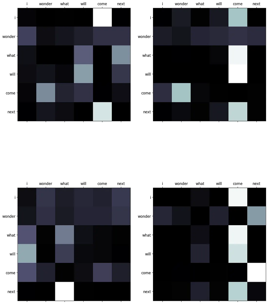
The next article will examine the Position-Wise Feed Forward Network.
Please don’t forget to like and follow for more! :)
Appendix
Display Attention
This function is used to display attention matrices.
def display_attention(sentence: list, translation: list, attention: Tensor,
                      n_heads: int = 8, n_rows: int = 4, n_cols: int = 2):
  """
    Display the attention matrix for each head of a sequence.

    Args:
        sentence:     German sentence to be translated to English; list
        translation:  English sentence predicted by the model
        attention:    attention scores for the heads
        n_heads:      number of heads
        n_rows:       number of rows
        n_cols:       number of columns
  """
  # ensure the number of rows and columns are equal to the number of heads
  assert n_rows * n_cols == n_heads

  # figure size
  fig = plt.figure(figsize=(15,20))

  # visualize each head
  for i in range(n_heads):

    # create a plot
    ax = fig.add_subplot(n_rows, n_cols, i+1)

    # select the respective head and make it a numpy array for plotting
    _attention = attention.squeeze(0)[i,:,:].cpu().detach().numpy()

    # plot the matrix
    cax = ax.matshow(_attention, cmap='bone')

    # set the size of the labels
    ax.tick_params(labelsize=12)

    # set the indices for the tick marks
    ax.set_xticks(range(len(sentence)))
    ax.set_yticks(range(len(translation)))

    ax.set_xticklabels(sentence)
    ax.set_yticklabels(translation)

  plt.show()
Scaling QK^T
To understand why scaling QK^T by √(d_key) has an impact on the softmax output, the same example sequences can be used. These examples can be passed through the multi-head attention until the point of calculating the dot product.
torch.set_printoptions(precision=2, sci_mode=False)

# convert the sequences to integers
sequences = ["I wonder what will come next!",
             "This is a basic example paragraph.",
             "Hello, what is a basic split?"]

# tokenize the sequences
tokenized_sequences = [tokenize(seq) for seq in sequences]

# index the sequences
indexed_sequences = [[stoi[word] for word in seq] for seq in tokenized_sequences]

# convert the sequences to a tensor
tensor_sequences = torch.tensor(indexed_sequences).long()

# vocab size
vocab_size = len(stoi)

# embedding dimensions
d_model = 8

# create the embeddings
lut = Embeddings(vocab_size, d_model) # look-up table (lut)

# create the positional encodings
pe = PositionalEncoding(d_model=d_model, dropout=0.1, max_length=10)

# embed the sequence
embeddings = lut(tensor_sequences)

# positionally encode the sequences
X = pe(embeddings)

# set the parameters

batch_size = X.size(0)
n_heads = 4
d_key = d_model//n_heads # 8/4 = 2
dropout=0.1

Wq = nn.Linear(d_model, d_model)    # query weights
Wk = nn.Linear(d_model, d_model)    # key weights
Wv = nn.Linear(d_model, d_model)    # value weights
Wo = nn.Linear(d_model, d_model)    # output weights

dropout = nn.Dropout(p=dropout)     # initialize dropout layer

# calculate query, key, and value tensors
Q = Wq(X)
K = Wk(X)
V = Wv(X)

# split each tensor into n-heads to compute attention

# query tensor
Q = Q.view(batch_size, -1, n_heads, d_key).permute(0, 2, 1, 3)
# key tensor
K = K.view(batch_size, -1, n_heads, d_key).permute(0, 2, 1, 3)
# value tensor
V = V.view(batch_size, -1, n_heads, d_key).permute(0, 2, 1, 3)
The next step is calculate QK^T, but it will be without a scale to start, and the values can be visualized before being passed through softmax.
# unscaled dot product
dot_prod = torch.matmul(Q,K.permute(0, 1, 3, 2))

# select the first sequence's first head
plt.imshow(dot_prod[0,0].detach(), cmap='gray')
plt.xlabel("$K^T$")
plt.ylabel("$Q$")
plt.colorbar()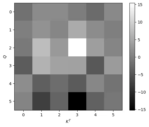
This first image shows the relation of each token in Q to its corresponding tokens in K^T. The highest value is around 15 and represented by white, and the lowest value is near -15 and represented by black. These will be the edges of the softmax function as well, which can be seen next.
plt.imshow(torch.softmax(dot_prod, dim=-1)[0, 0].detach())
plt.xlabel("$K^T$")
plt.ylabel("$Q$")
plt.colorbar()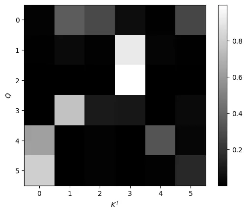
The highest values from the previous image are the highest values in the new image, with the rest of the values falling below 0.1. This shows the potential danger of not scaling the dot product because these values can result in extremely small gradients that can disrupt training. Now, the next image shows how scaling helps prevent this by dividing by √(d_key).
# calculate the scaled dot product
scaled_dot_prod = torch.matmul(Q, K.permute(0, 1, 3, 2)) / math.sqrt(d_key)

# first sequence's first head
plt.imshow(scaled_dot_prod[0,0].detach())
plt.xlabel("$K^T$")
plt.ylabel("$Q$")
plt.colorbar()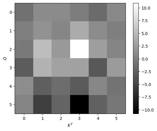
This image is the same as the original one, but the color bar has shifted according to the scale, falling between approximately 10 and -10. The difference will be seen once these values are normalized with softmax. Since there is not such a large range, more values will fall closer to the middle of the probability distribution, which is ideal.
plt.imshow(torch.softmax(scaled_dot_prod, dim=-1).detach()[0,0])
plt.xlabel("$K^T$")
plt.ylabel("$Q$")
plt.colorbar()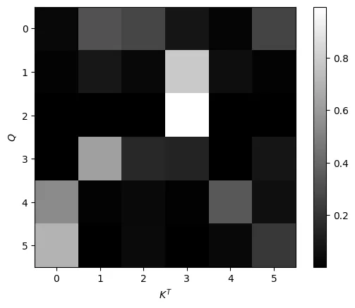
This image shows how scaling the dot product makes the output of the softmax function less focused around 0 and 1. There are more gray values instead of mostly black or white. Values that were closer to zero or one in the unscaled distribution are now getting closer to the middle of the distribution.
Supplementary Images of Attention
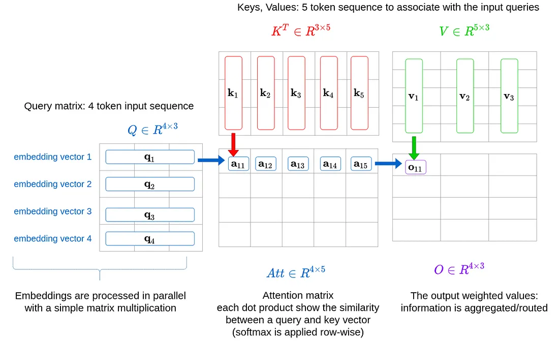
This is an additional view of how multi-head attention is calculated. The image below has examples of how the softmax is calculated between different representations of the same sequence.

